PDF transformations Link to heading

While reading new [book]¹ by Bishop I came across pdf transformation topic. It turned out to be counter-intuitive that we need not only transform the pdf by the selected function, but also multiply it by the derivative of the inverse function w.r.t. substituted variable. While delving into the details of this topic, I found the following sources to be quite useful: [2]², [3]³, [4]⁴, [5]⁵.

Introduction Link to heading

Assume that we have random variable $X$ that has a continuous distribution on an interval $S \in \mathcal{R}$, its probability density function $f(x)$ is known. Suppose that we have a differentiable function $y$ from $S$ to $T \in \mathcal{R}$ and we apply this function to random variable $X$. We end up having a new random variable $Y = y(X)$. The question is how can we find the distribution of our random variable $Y$?

The main theorem Link to heading

We know, by definition of probability that:

Now, if $X = a$ the derived random variable $Y = y(a)$ and if $X = b$, $Y = y(b)$. Hence:

In the last step we used the integration by substitution method, $x(y)$ is $x$ expressed in terms of $y$.

The right-hand integrand $f(x(y))\frac{dx}{dy}$ is expressed wholly in terms of y, so can be replaced by function $g(y)$:

making it obvious that $g(y)$ is the pdf associated with $Y$.

Now, taking the derivative, we have

Here we have an absolute value because the formula is the same for increasing or decreasing $g$.

While being compact, this formula is less clear. We must remember that $x$ on the ride side should be written in terms of $y$, but since we originally express $y$ in terms of $x$: $Y = y(X)$, the inverse function should be used there.

To be a little bit more explicit let’s rewrite this equation using arbitrary function $r$: $y = r(x)$ applied to variable $x$, and giving back variable $y$, the aforementioned formula can be rendered as follows:

What this formula states is that any density $g(y)$ can be obtained from a fixed density $f(x)$.

Example 1 Link to heading

Suppose that $Y = a + bX$, $a \in \mathcal{R}$ and $b \in \mathcal{R} \backslash \{0\}$, the distribution of $X$ is known: $f(x)$. What is the pdf of $Y$?

Since $r(x) = y = a + bx$, we can find inverse function to be $r^{-1}(y) = x = \frac{y - a}{b}$ and the derivative $\frac{dx}{dy} = \frac{1}{b}$.

Then $g(y) = f(\frac{y - a}{b})\frac{1}{|b|}$.

Example 2 Link to heading

Suppose that $f(x) = 2 x, x \in [0, 1)$ and $y(x) = x^2$.

First, derive the inverse of the function $x(y) = \sqrt{y}$.

Now, having:

we can find $g(y)$ to be:

So after applying transformation $y(x) = x^2$ to random variable $X$ the function $y(x)$ transforms the triangular distribution into the uniform one.

Example 3 Link to heading

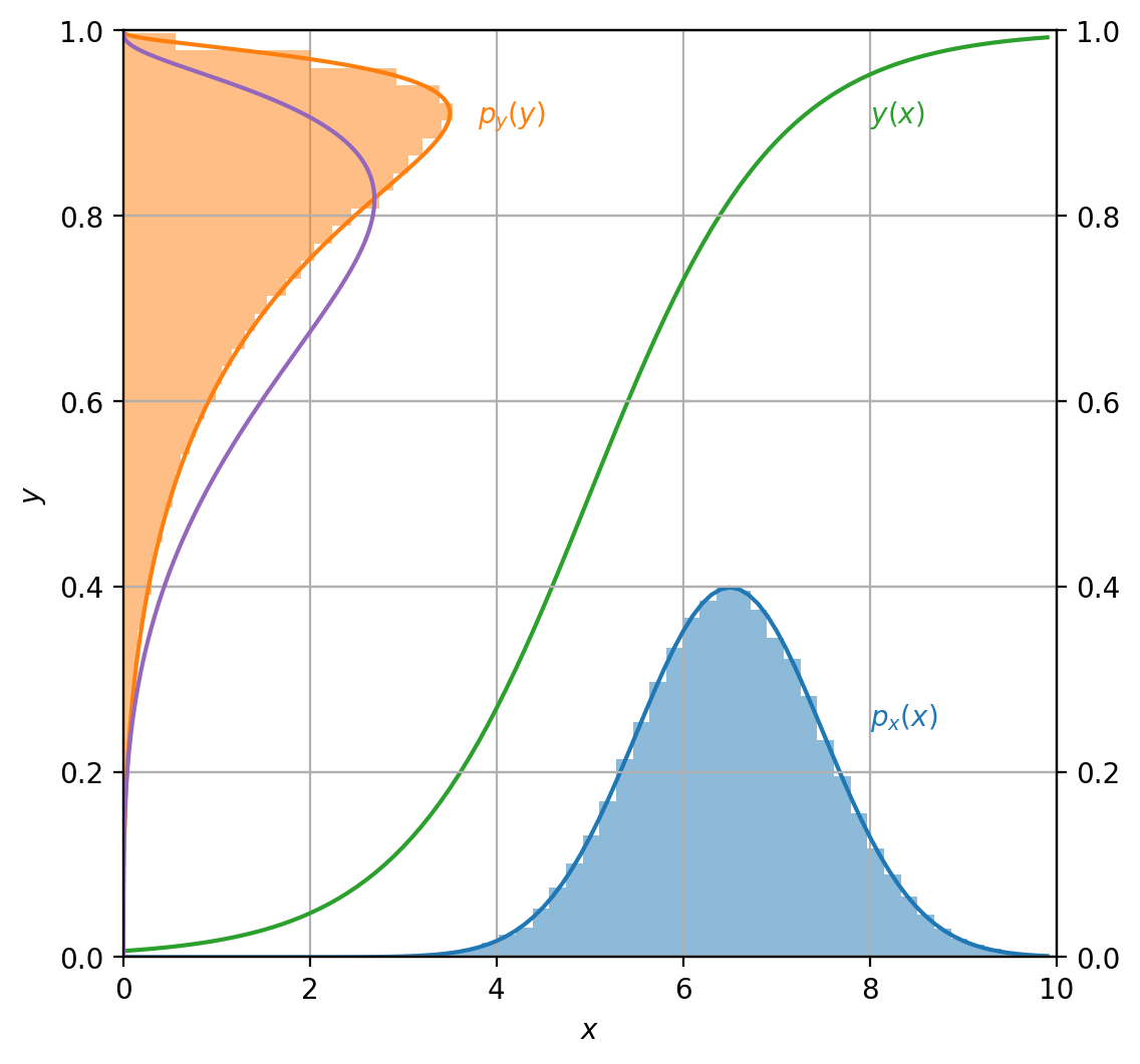
Given random variable $X \sim \mathcal{N}(6.5, 1.)$ we apply to it transformation function $y(x)$ specified as:

Let $Y = y(X)$, and $p(y)$ be the pdf associated with $Y$. What is the pdf of $p(y)$?

Let’s solve the problem using sympy:

import sympy as sp
x = sp.Symbol('x', positive=True)
y = sp.Symbol('y')

y_x = 1. / (1. + sp.exp(5 - x))
x_y = sp.solve(y_x - y, x)[0]

dx_dy = x_y.diff(y).simplify()

# print(sp.latex(x_y), sp.latex(dx_dy))

After solving for $y$ and finding the derivative we got:

import sympy.stats

X = sp.stats.Normal('x', 6.5, 1)
pdf_x = sp.stats.density(X)(x)

pdf_y_simple_transform = pdf_x.subs({x:x_y})
pdf_y = (pdf_x * dx_dy).subs({x:x_y})
# print(sp.latex(pdf_y))

Giving the following $p(y)$:

Now let’s plot everything. First let’s plot $p(x)$ and draw samples from $X$ distribution, plotting the histogram of their values (blue).

Next, let’s apply the function $y(x)$ to each sample from the drawn set and plot its histogram too (orange).

If we substitute $x$ by $y$ in $p(x)$, we will obtain a purple curve. However, this curve does not agree with the histogram!

The correct curve for $p(y)$ density is shown in orange. In this case, in addition to substitution, we multiplied the result by $\frac{dx}{dy}$ to obtain the correct result.

import numpy as np
from scipy.stats import norm

# lambdify pdfs
p_x = sp.lambdify(x, pdf_x)
p_y_simple_transform = sp.lambdify(y, pdf_y_simple_transform)
p_y = sp.lambdify(y, pdf_y)

# lambdify functions
y_x_func = sp.lambdify(x, y_x, modules = ["numpy"])
x_y_func = sp.lambdify(y, x_y)
dx_dy_func = sp.lambdify(y, dx_dy)

x_interval = np.arange(0, 10, 0.1)
y_interval = np.linspace(0.0, 1.0, 1000, endpoint=False)

# sample X from our distribution
X_sampled = norm(6.5, 1.).rvs(size = 100000)
# transform the values
Y = y_x_func(X_sampled)

import matplotlib.pyplot as plt
%matplotlib inline
%config InlineBackend.figure_format='retina'

fig, ax = plt.subplots(1, 1, figsize=(6, 6))
ax.plot(x_interval, p_x(x_interval), c='tab:blue')
ax.hist(X_sampled, density=True, bins = 50, color='tab:blue', alpha = 0.5)
ax.plot(x_interval, y_x_func(x_interval), c='tab:green')
ax.set(ylim=[0, 1], xlim=[0, 10])
ax.text(8, 0.25, '$p_x(x)$', color='tab:blue')
ax.text(8, 0.9, '$y(x)$', color='tab:green')
ax.grid(axis='both')
ax.set(xlabel='$x$')
ax.set(ylabel='$y$')

ax2 = ax.twinx()
ax2.hist(Y, density=True, bins = 50, orientation="horizontal", color='tab:orange', alpha = 0.5)
ax2.plot(p_y(y_interval), y_interval, c='tab:orange')
ax2.plot(p_y_simple_transform(y_interval) / np.trapz(p_y_simple_transform(y_interval), y_interval), y_interval, c = 'tab:purple')
ax2.set(ylim=[0, 1])
ax2.text(3.8, 0.9, '$p_y(y)$', color='tab:orange')
ax2.grid(axis='both')

Example 4 Link to heading

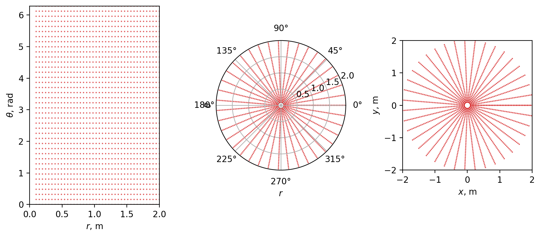
For the next example, let’s consider coordinate transform.

The polar coordinate transforms two numbers $(r, \theta)$, where radial distance $r \in [0, \inf)$ and polar angle $\theta \in [0, 2\pi)$ to a point on a plane.

Evaluating the derivatives we get:

We can view this transformation as a multivariate change of variables. In such a case instead of $\frac{dx}{dy}$ we use the determinant of Jacobian ($\mathbf{J}$) that describes how the volume changes under the transformation.

Now, if we sample a polar coordinate $(r, \theta)$ with probability $f(r, \theta)$, then the distribution $g(x, y)$ is given by:

Now let’s repeat an experiments. First let’s take a look how the uniform grid changes after applying $x(r, \theta)$ and $y(r, \theta)$.

import matplotlib.pyplot as plt
import numpy as np
from scipy.stats import uniform, multivariate_normal

# sample points uniformly in polar space
r_interval = np.linspace(1e-1, 2, 40)
theta_interval = np.linspace(0.0, 2 * np.pi, 40)
r, theta = np.meshgrid(r_interval, theta_interval)

# transform
x, y = r * np.cos(theta), r * np.sin(theta)

fig = plt.figure(figsize=(9, 4))
ax1 = fig.add_subplot(131)
ax2 = fig.add_subplot(132, polar=True)
ax3 = fig.add_subplot(133)


ax1.scatter(r, theta, s = 10, edgecolor='none', alpha = 0.75, marker='.', c = 'tab:red')
ax1.set(xlim = [0, 2], ylim=[0, 2 * np.pi], xlabel='$r$, m', ylabel='$\\theta$, rad')
ax2.scatter(theta, r, s = 10, edgecolor='none', alpha = 0.75, marker='.', c = 'tab:red')
ax2.set_rmax(2)
ax2.set_rticks([0.5, 1, 1.5, 2])
ax2.set(xlabel='$r$', ylabel='$\\theta$')

ax3.scatter(x, y, s = 10, edgecolor='none', alpha=0.75, marker='.', c = 'tab:red')
ax3.set(xlim =[-2, 2], ylim=[-2, 2], aspect='equal', xlabel='$x$, m', ylabel='$y$, m')

fig.tight_layout()

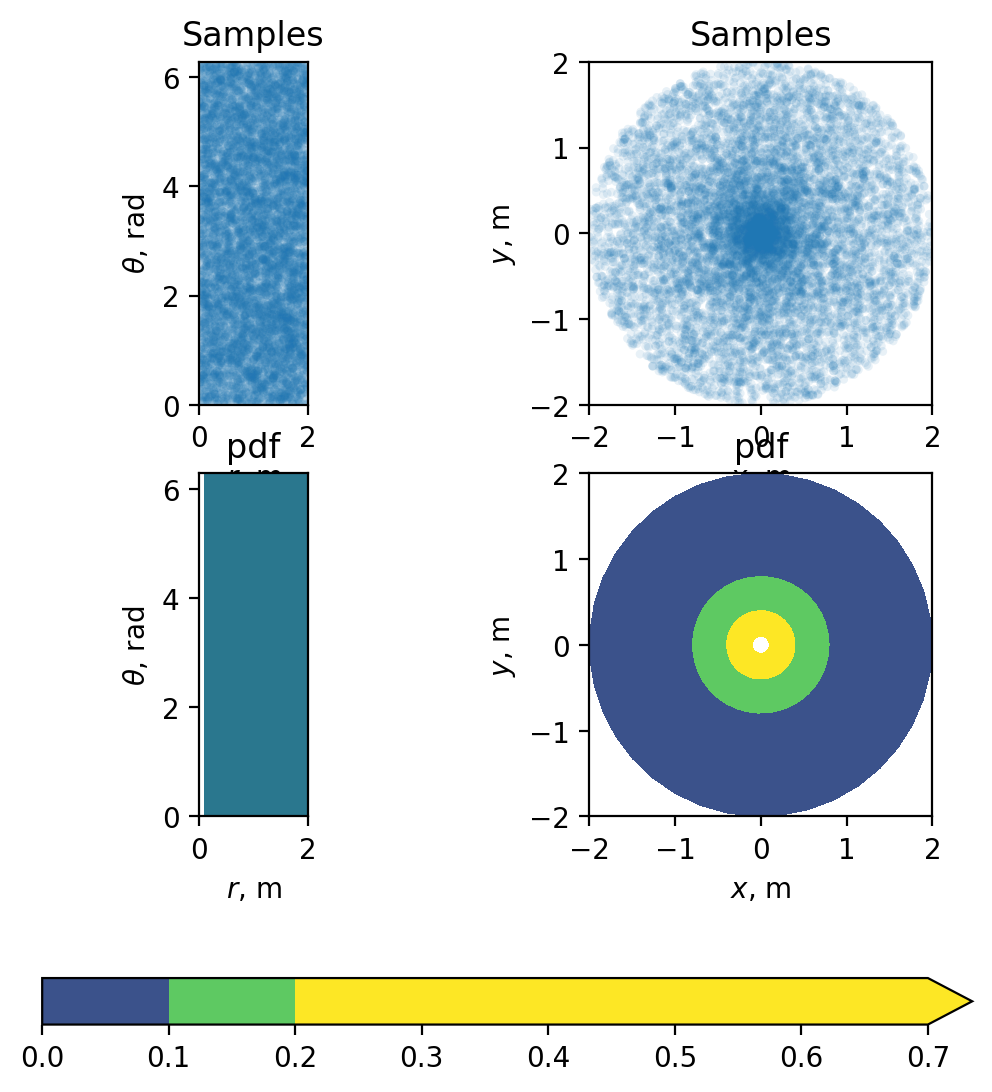
And finally, let’s draw samples from our $f(r, \theta)$ distribution, apply our transform, and plot the transformed samples. The top row of the plot displays the transformed samples, while the bottom row shows the $f(r, \theta)$ and $g(x, y)$ pdfs.

# pdf for r, theta multivariate distribution
f_rtheta = uniform(0, 2).pdf(r) * uniform(0, 2 * np.pi).pdf(theta)
g_xy = f_rtheta / r

fig, ax = plt.subplots(2, 2, figsize = (6, 7))
ax1 = plt.subplot(221)
ax2 = plt.subplot(222)
ax3 = plt.subplot(223)
ax4 = plt.subplot(224)

r_sampled, theta_sampled = uniform(0, 2).rvs(size=10000), uniform(0, 2 * np.pi).rvs(size=10000)
x_sampled, y_sampled = r_sampled * np.cos(theta_sampled), r_sampled * np.sin(theta_sampled)

ax1.scatter(r_sampled, theta_sampled, s = 10, edgecolor='none', alpha = 0.1)
ax1.set(xlim = [0, 2], ylim=[0, 2 * np.pi], aspect='equal', xlabel='$r$, m', ylabel='$\\theta$, rad', title='Samples')
ax2.scatter(x_sampled, y_sampled, s = 10, edgecolor='none', alpha=0.1)
ax2.set(xlim = [-2, 2], ylim=[-2, 2], aspect='equal', xlabel='$x$, m', ylabel='$y$, m', title='Samples')
ax3.contourf(r, theta, f_rtheta, vmin=0, vmax = 0.2)
ax3.set(xlim = [0, 2], ylim=[0, 2 * np.pi], aspect='equal', xlabel='$r$, m', ylabel='$\\theta$, rad', title='pdf')
cf = ax4.contourf(x, y, g_xy, vmin=0, vmax = 0.2, extend='max', cmap='viridis')
ax4.set(xlim = [-2, 2], ylim=[-2, 2], aspect='equal', xlabel='$x$, m', ylabel='$y$, m', title='pdf')
fig.colorbar(cf, ax=(ax1, ax2, ax3, ax4), orientation='horizontal')

References Link to heading