Particle filter Link to heading

In this post I would like to show the basic implementation of the Particle filter for robot localization using distance measurements to the known anchors, or landmarks. So why particle filter is so widely used? It’s widespread application lies in its versatile nature and universalism. The filter is able to:

• Work with nonlinearities.
• Handle non-gaussian distributions.
• Easily fuse various information sources.
• Simulate the processes.

My sample implementation takes less then 100 lines of Python code and can be found here.

Idea Link to heading

The idea of the particle filter is to represent the probability distribution by a set $X$ of random samples drawn from the original probability distribution. These samples usually called particles. Every particle $x^{(i)}_t$ can be seen as the hypothesis about what true state can be at time $t$.

In ideal world, the likelihood of getting a hypothesis $x^{(i)}_t$ shall be proportional to its Bayes posterior:

The particle filter is the recursive one. That means that belief at time $t$ is being computed from the belief one time step earlier, $t-1$. Since the belief is represented by the particle set $X$, then the particles from $X_{t-1}$ can be transformed into the set $X_t$ based on system model.

Steps Link to heading

Each particle filter iteration cycle can be broken into three steps:

1. Prediction. Generate the particle set $X_t$ based on the particle set $X_{t-1}$ and the control $u_t$. If it is the initialization, then the particle set have to be generated across all possible states. Usually on this step some noise is injected into the model to accomodate for noise in control and to make particle set more distributed.
2. Correction. Calculate the importance factor, or weight of each particle. The importance factor is the probability to get the measurement $z_t$ given the hypothesis, or particle $x_t$: $w^{(i)}_t = p(z_t | x^{(i)}_t)$. If more than one measurement is available, say $M$, then all these measurements should be multiplied under the assumption that they are independent: $w^{(i)}_t = \prod_{j=1}^M p(z_{t,j} | x^{(i)}_t)$. Normalize the particle weights: $w_{t}^{(i)}={\frac {{ {w}}_{t}^{(i)}}{\sum _{i=1}^{N}{{w}}_{t}^{(i)}}}$. The set of weighted particles represents the filter belief.
3. Resampling. It is done through replacing when the more unlikely hypothesis with more likely ones. The probability of drawing each particle is given by its relative importance weight (w.r.t the whole set). The idea of resampling is similar to the idea in volutionary algorithms: only the fittest ones should survive.

Notes:

1. It is not always the best idea to sample the particles across all possible state space on the initialization. Sometimes it is better to wait for few available measurements and sample from $p(z_t|m)$, where $m$ – is the map.
2. The resampling process is computational extensive. Therefore it is recommended to resample only when the effective number of particles is less than the given threshold $N_X$. It is shown, that the effective number of particles can be approximated as: $\hat {N}_{\mathit {eff}}={\frac {1}{\sum _{i=1}^{N}\left(w_{k}^{(i)}\right)^{2}}}$. This formula reflects the variance of particle weights.

Importance Sampling Link to heading

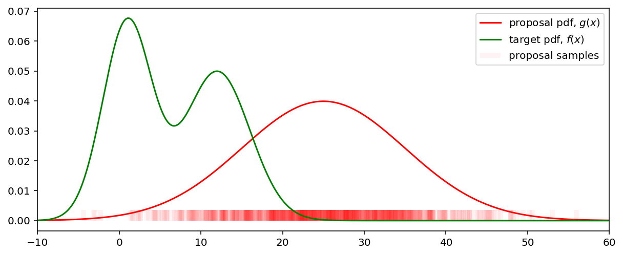
To understand the idea behind importance sampling more clearly let’s reformulate the problem: say we would like to get a sample from target distribution $f$, from which direct sampling is very hard or even impossible. However, we are able to generate the samples from some probability density function $g$, called proposal distribution.

What resampling step is able to do is to generate a new set of particles distributed according to the density function $f$ given the set of particles distributed according to density $g$.

To illustrate this let’s generate samples from density $g$. The samples, drawn from $g$ are shown on the bottom of the plot.

N_samples = 1000
proposal_mean = 25
proposal_std = 10.0
xfrom, xto = -10, 60

def target_pdf(x):
    return 0.5 * norm.pdf(x, 1.0, 3.0) + 0.5 * norm.pdf(x, 12.0, 4.0)

proposal_samples = np.random.normal(proposal_mean, proposal_std, size=N_samples)

fig, ax = plt.subplots(1, 1, figsize=(10, 4), sharex = True)
x = np.linspace(xfrom, xto, 1000)
ax.plot(x, norm.pdf(x, proposal_mean, proposal_std), label='proposal pdf, $g(x)$', c='red')
ax.plot(x, target_pdf(x), label='target pdf, $f(x)$', c='green')
# plot rug plot
rel_rug_height = ax.get_ylim()[1] / 20.0
ax.vlines(proposal_samples, [0] * N_samples, [rel_rug_height] * N_samples, 
          alpha=0.05, colors='red', label='proposal samples', linewidths=5.0)
ax.set_xlim([xfrom, xto])
ax.legend()

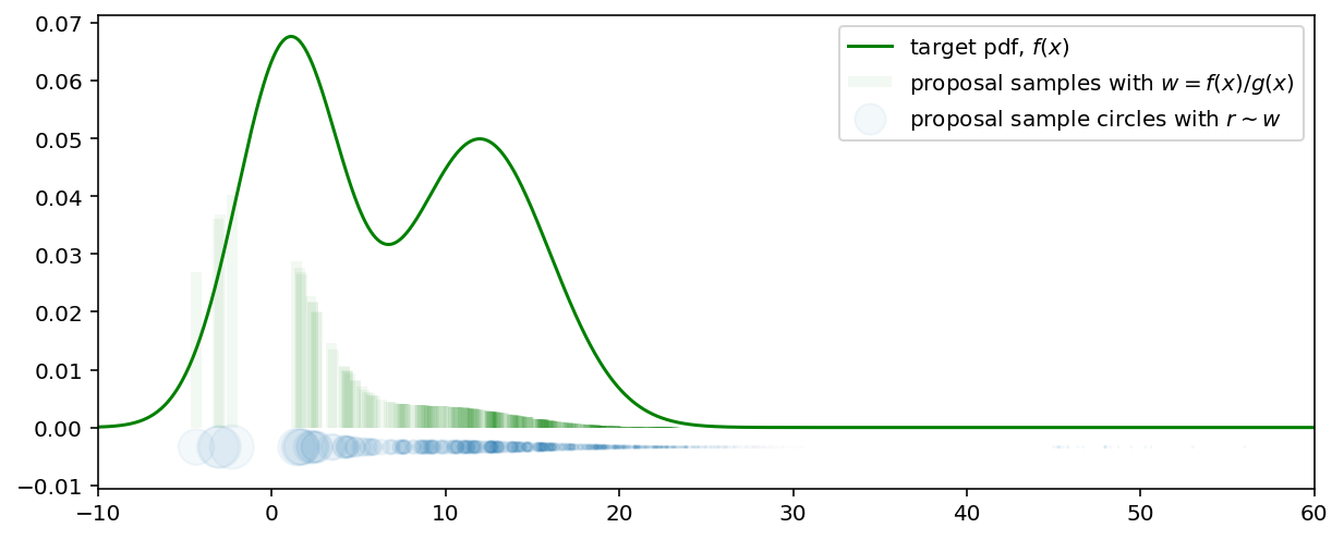
Samples from $f$ are obtained by attaching weights $w = f(x) / g(x)$ to each sample, drawn from $g$. The following plot shows the proposal samples with their associated weights (the height of the vertical lines). Some weights became equal to zero while the others are significantly increased. For example, in spite of the fact that the proposal density in range $(20, 30)$ is high, due to the weighing these samples became insignificant.

The combination of color intensity and the height of the vertical bars can be considered as the target probability density function. The more intensive and higher the vertical bars - the more probable the neighbourhood samples $x$ around it. As an alternative, weights are shown as circles where the radius of the circle reflects the particle weight and the circle color intensity due to the overlapping - is their density in the given region.

target_weights = target_pdf(proposal_samples) / norm.pdf(proposal_samples, proposal_mean, proposal_std)

fig, ax = plt.subplots(1, 1, figsize=(10, 4))
ax.set_xlim([xfrom, xto])
ax.vlines(proposal_samples, [0] * N_samples, target_weights / np.sum(target_weights), 
          alpha=0.05, colors='green', label='proposal samples with $ w = f(x) / g(x)$', linewidths=5.0)
x = np.linspace(xfrom, xto, 1000)
ax.plot(x, target_pdf(x), label='target pdf, $f(x)$', c='green')
ax.scatter(proposal_samples, [ax.get_ylim()[0]] * N_samples, 
           sizes=target_weights / np.sum(target_weights) * 10000, alpha=0.05,
           label="proposal sample circles with $r \sim w$")
    
ax.legend()

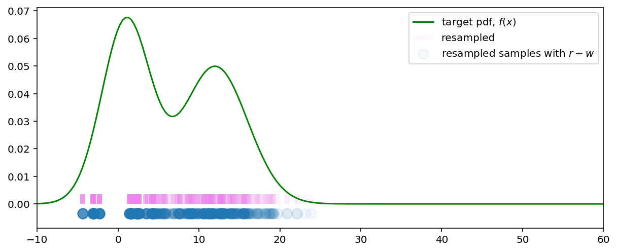
Now, if we resample from the weighted samples distribution we get the samples from our target distribution (as $N \xrightarrow{}\infty$):

def systematic_resample(weights, samples):
    weights, samples, n_samples = np.array(weights), np.array(samples), len(samples)
    weights /= np.sum(weights)
    r, c, i = np.random.uniform(0.0, 1.0 / N_samples), weights[0], 0
    resampled = []
    for m in range(0, n_samples):
        U = r + m / n_samples
        while c < U:
            i += 1
            c += weights[i]
        resampled.append(deepcopy(samples[i]))
    return resampled

fig, ax = plt.subplots(1, 1, figsize=(10, 4))  
x = np.linspace(xfrom, xto, 200)
ax.plot(x, target_pdf(x), label='target pdf, $f(x)$', c='green')
target_samples = systematic_resample(target_weights, proposal_samples)
rel_rug_height = ax.get_ylim()[1] / 20.0
ax.vlines(target_samples, [0] * N_samples, [rel_rug_height] * N_samples, 
          alpha=0.05, colors='violet', label='resampled', linewidths=5.0)
ax.scatter(target_samples, [ax.get_ylim()[0]] * N_samples, 
           s=100, alpha=0.05,
           label="resampled samples with $r \sim w$")

ax.legend()
ax.set_xlim([xfrom, xto])
plt.show()

Particle filter implementation Link to heading

Now, having all key concepts explained, we can write the particle filter implementation for robot localization. The filter state consists of:

• robot position - $(x, y)$.
• robot heading angle - $\theta$.

The robot moves along a map and measures the distances to the known landmarks, or anchors, when they are within its sense range.

The robot distance measurements to the landmarks and its motion controls are not perfect. To take that into account I inject the noises in particle filter process in the following forms:

• For predict step - the control $u_t$ that consists of $(\delta d, \delta \theta)$ is additionally pertrubated with random noise, $N(0, \sigma_{motion})$ and $N(0, \sigma_{\theta})$.
• For correction step. Whenever the robot measures the distances to the known landmark $n$, we can asses the measurement likelihood given our state $(x, y, \theta)$. Having the predicted $\hat{d} = \sqrt{(x - x_{landmark})^2 + (y - y_{landmark})^2}$ and measured $d_n$ distances, and the measurement noise $\sigma_d$ the likelihood can be calculated as: $$p(z_n|x_t) = {\frac {1}{\sigma_d {\sqrt {2\pi }}}}e^{-{\frac {1}{2}}\left({\frac {\hat{d}-d_{n} }{\sigma_d }}\right)^{2}}$$ The current particle weight have to be multiplied with $p(z_n|x_t)$ for each available measurement.

Then the weights have to be renormalized, particles - resampled, if it is neccessary. This process continues to evolve in iterative manner.

Animation Link to heading

To test the code and view the particle filtering process in action you can simply execute run.py script:

python3 run.py

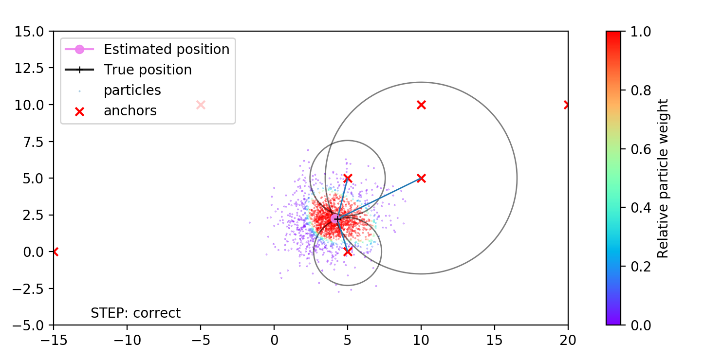
In the following animation the robot moves along a circle and measures the distances to anchors that are marked with red crosses. The true robot position is shown with black plus sign. The blue lines, connecting the robot and the anchors - true distance measurements between the robot and the anchors, the grey circles - the measured distances between robot and anchor. Feel free to experiment with configuration and add new types of measurements (for example the heading w.r.t to the anchors, or absolute motion heading).