Quite often we want to sample from distributions that have computationally untractable CDF. To draw samples from them the numerical procedures are used. In the following note I would like to demonstrate few approaches for one particular example: having 2D robot perception and a map we want to sample most probable poses of this robot. This problem often emerges during initialization or re-initialization of the estimated robot pose when the filter diverged or needs to be initialized from scratch and we want to guarantee the fast convergence.
Most of the approaches discussed in this post come from [1].
Rejection sampling Link to heading
Suppose we want to sample from an arbitrary distribution $p(\mathbf{z})$, which pdf has a complex form and we can not sample directly. However, we can easily calculate the actual value of $p(\mathbf{z})$ for any given $\mathbf{z}$ up to some normalizing constant $Z$:
$$ p(\mathbf{z}) = \frac{1}{Z_p}\tilde{p}(\mathbf{z}), $$where $\tilde{p}(\mathbf{z})$ can be readily evaluated, but $Z_p$ is unknown. The idea is as follows:
- Draw a sample $z_0$ from a proposal distribution $q(\mathbf{z})$.
- Draw a sample $u_0$ from the uniform distribution over $[0, kq(z_0)]$.
- If $u_0 \leq \tilde{p}(z_0)$ then the sample $z_0$ is accepted, otherwise it is rejected.
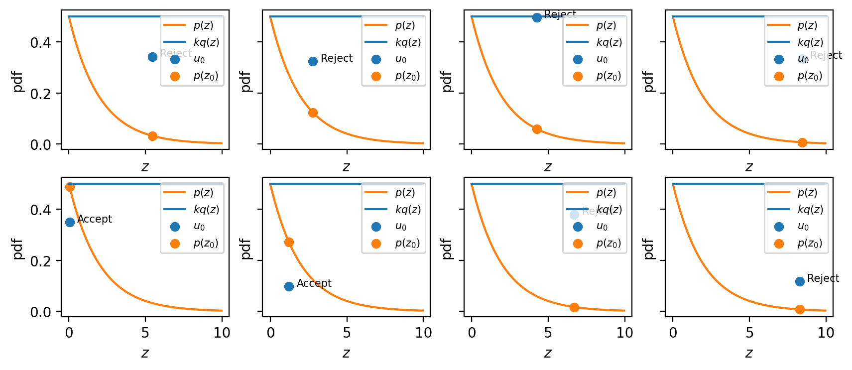
Here is the visualization of the algorithm. First we sample a random number $z_0$ from the proposal distribution (along horizontal). Then we sample a second number $u_0$ (along vertical), the upper bound of $u_o$ is equal to $kq(z_0)$, which makes perfects sense - our proposal distribution should cover all the distribution we would like to sample from. As a last step we check whether or not $u_0$ is above or under $p(z_0)$. If it is under, then we are within our target distribution and the sample should be retained.
import matplotlib.pyplot as plt
import numpy as np
from scipy.stats import uniform

np.random.seed(100)

exp_pdf = lambda x, Lambda=0.5: Lambda * np.exp(-Lambda * x)
uniform_pdf = uniform(0, 10).pdf

samples = []
# sample from our proposal distribution
z0 = np.random.uniform(0, 10, size = 1000000)
# sample from the uniform over our range
# since our proposal is uniform, we know the pdf of each sample = 0.1
# k should be equal to 5 to make sure that k * q(z) >= p(z)
k = 5.
u0 = np.random.uniform(0, k * 0.1, size = 1000000)
samples = z0[u0 <= exp_pdf(z0)]

xx = np.arange(0, 10, 0.05)
fig, axes = plt.subplots(2, 4, figsize = (10, 4), sharex = True, sharey = True)
for i, ax in enumerate(axes.flatten()):
    ax.plot(xx, exp_pdf(xx), label="$p(z)$", c="tab:orange")
    ax.plot(xx, uniform_pdf(xx) * k, label="$kq(z)$", c="tab:blue")
    z = z0[i]
    u = u0[i]
    ax.scatter([z], [u], label = "$u_0$")          # that is our
    ax.scatter([z], [exp_pdf(z)], label = "$p(z_0)$") # that is the pdf we want to sample from
    ax.text(z + 0.5, u, f'{"Accept" if u <= exp_pdf(z) else "Reject"}', fontsize = 7.5)
    ax.legend(loc="upper right", fontsize = 7.5)
    ax.set(xlabel = "$z$", ylabel = "pdf")
It is worth to note several things:
- The original values of $z$ are accepted with probability $\frac{p(z)}{kq(z)}$. If we take the integral it becomes obvious that the fraction of points that are rejected depends on the ratio of the area under the unnormalized distribution $p(z)$ to the are under the curve $kq(z)$.
- As a consequence of this the proposal distribution should be as close as possible to the target distribution to achieve the high acceptance rate.
- If we sample from uniform distribution, we can get rid of $kq(z)$ evaluation, since it is constant.
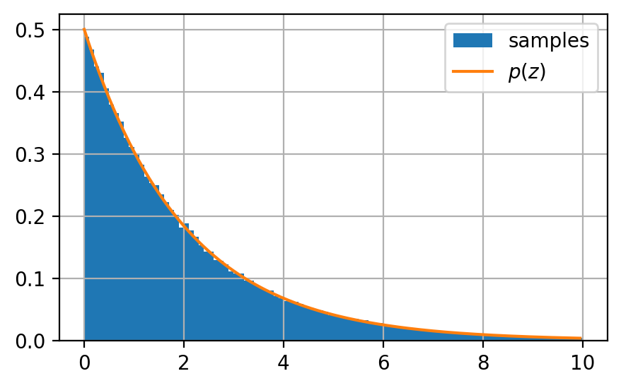
Let’s confirm that our samples reflect the original distribution we wanted to sample from:
fig, ax = plt.subplots(1, 1, figsize = (5, 3))
xx = np.arange(0, 10, 0.05)
ax.hist(samples, density=True, stacked=True, bins = 100, label="samples");
ax.plot(xx, exp_pdf(xx), label="$p(z)$", c="tab:orange")
ax.grid()
ax.legend()
MCMC sampling Link to heading
Since direct sampling from a multidimensional distribution is hard, another method is required. Such a family of methods is called Markov chain Monte Carlo (MCMC), which allows sampling from a large class of distributions and scales well for high-dimensional spaces.
The idea is quite close to the rejection sampling, but this time we keep a record of the current state $\mathbf{z}^{(\tau)}$, and the proposal distribution $q(\mathbf{z}|\mathbf{z}^{(\tau)})$ depends on this current state, and the sequence of samples forms a Markov chain.
At each cycle of the algorithm, a candidate sample $\mathbf{z}^*$ is generated and then accepted based on an appropriate criterion.
Metropolis algorithm Link to heading
In Metropolis algorithm, it is assumed that the proposal distribution is symmetric and the candidate sample is accepted with probability:
$$ A(\mathbf{z}^*, \mathbf{z}^{(\tau)}) = \min\left( 1, \frac{\tilde{p}(\mathbf{z}^*)}{ \tilde{p}(\mathbf{z}^{(\tau)})} \right). $$The simplest method to achieve this is by selecting a random number $\mathbf{u}$ from a uniform distribution and then accepting the sample if $A > u$. Notes:
- In contrast to rejection sampling, the candidate is kept not only if the sampled value falls “within” our target distribution, but also if the next drawn sample leads to an increase of the $p(\mathbf{z})$.
- If proposal distribution is not symmetric, then the Metropolis-Hastings criterion shall be used, that applies the correction term.
Gibbs Sampling Link to heading
The concept of Gibbs sampling is relatively straightforward: at each iteration, we update the value of one variable by sampling from its conditional distribution given the values of the other variables. This process iterates through each variable in a cyclical manner.
The practical utility of Gibbs sampling relies on the ease of sampling from the conditional distributions $p(z_k|\mathbf{z}_{\not k})$. Two effective approaches are:
- Utilizing rejection sampling techniques, as previously discussed.
- Precomputing $p(\mathbf{z})$ on a multidimensional grid and subsequently leveraging this grid to compute the conditional probability density functions.
Sampling Link to heading
Now let’s actually sample the robot poses given our perception. For a simplicity let’s assume that our map consists of 5 points and we also perceive same 5 points, but in robot coordinate system.
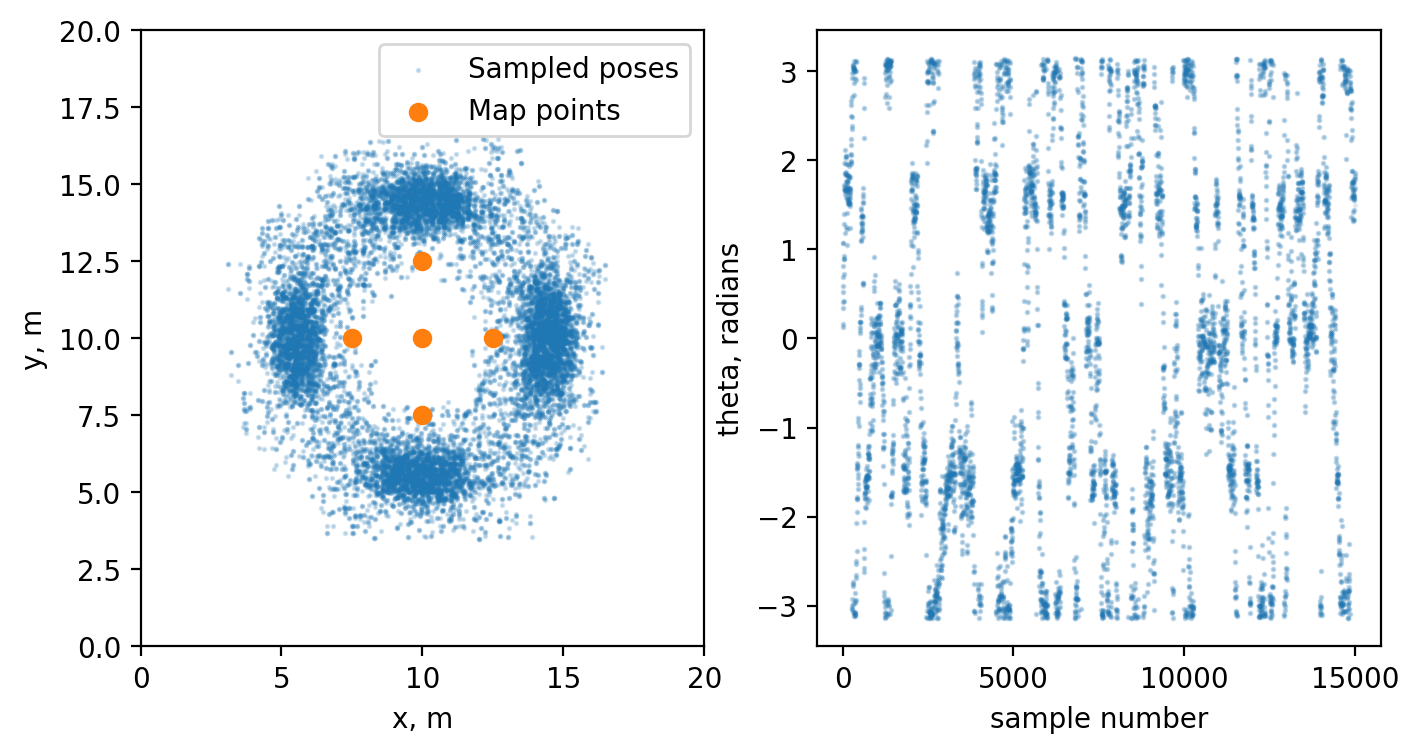
Option 1 Link to heading
The first option is to directly sample from our uniform distribution and check whether or not the next sample should be discarded using Metropolis algorithm, while iterating through our state variables.
import numpy as np
from scipy.spatial import KDTree
from scipy.stats import norm

def norm_pdf(x, mu, sigma):
    """Calculates normal pdf for sample x given parameters mu and sigma."""
    variance = sigma**2
    numerator = x - mu
    denomenator = 2*variance
    pdf = ((1/(np.sqrt(2*np.pi)*sigma))*np.exp(-(numerator**2)/denomenator))
    return pdf

def transform_to_world(perception, pose):
    """Resolves perception in world coordinate frame based on current pose."""
    x, y, theta = pose
    c, s = np.cos(theta), np.sin(theta)

    perception_world = np.zeros_like(perception)
    for i, p in enumerate(perception):
        perception_world[i, :] = (p[0] * c - p[1] * s + x, p[0] * s + p[1] * c + y)

    return perception_world

def estimate_perception_logpdf(perception, x, y, theta, sigma=1.):
    """Calculates pdf of perception given the pose."""
    perception_world = transform_to_world(perception, (x, y, theta))
    distances, _ = tree.query(perception_world, k=1)
    w = np.sum(np.log(norm_pdf(distances, 0., sigma)))
    return w

def gibbs_sample_step(perception, current_logpdf, current_pose, dim_to_sample, n_attempts=500):
    """Tries to draw the next sample based on current pose, perception and current pdf."""
    x, y, theta = current_pose
    for i in range(0, n_attempts):
        if dim_to_sample == 'x':
            x = np.random.uniform(0, 20)
        elif dim_to_sample == 'y':
            y = np.random.uniform(0, 20)
        elif dim_to_sample == 'theta':
            theta = np.random.uniform(-np.pi, np.pi)

        pose_logpdf = estimate_perception_logpdf(perception, x, y, theta)
        k = pose_logpdf - current_logpdf
        if k >= 0.0 or np.log(np.random.uniform()) < k:
            return (x, y, theta), pose_logpdf

    return (x, y, theta), pose_logpdf


# Define world points
map_points = np.array([[10., 7.5], [7.5, 10.], [10., 10.], [12.5, 10.], [10., 12.5]])
tree = KDTree(map_points)
# Define robot perception of the world
perception = [[2., 0], [4.5, -2.5], [4.5, 0.], [4.5, 2.5], [7., 0]]

samples = []
current_pose = (np.random.uniform(0, 20), np.random.uniform(0, 20), np.random.uniform(-np.pi, np.pi))
pose_logpdf = -np.inf
np.random.seed(100)
# sample the robot poses using gibbs sampling procedure
for i in range(0, 5000):
    current_pose, pose_logpdf = gibbs_sample_step(perception, pose_logpdf, current_pose, 'x')
    samples.append(current_pose)
    current_pose, pose_logpdf = gibbs_sample_step(perception, pose_logpdf, current_pose, 'y')
    samples.append(current_pose)
    current_pose, pose_logpdf = gibbs_sample_step(perception, pose_logpdf, current_pose, 'theta')
    samples.append(current_pose)

fig, ax = plt.subplots(1, 2, figsize = (8, 4))
samples = np.array(samples)
ax[0].scatter(samples[:, 0], samples[:, 1], s=1, alpha = 0.2, c="tab:blue", label="Sampled poses")
ax[0].scatter(map_points[:, 0], map_points[:, 1], c='tab:orange', label="Map points")
ax[0].set(xlim=(0, 20), ylim=(0, 20), xlabel="x, m", ylabel="y, m")
ax[0].legend()
ax[1].scatter(np.arange(0, len(samples)), samples[:, 2], s=1, alpha = 0.1, c="tab:blue", label="Sampled poses theta")
ax[1].set(xlabel="sample number", ylabel="theta, radians")
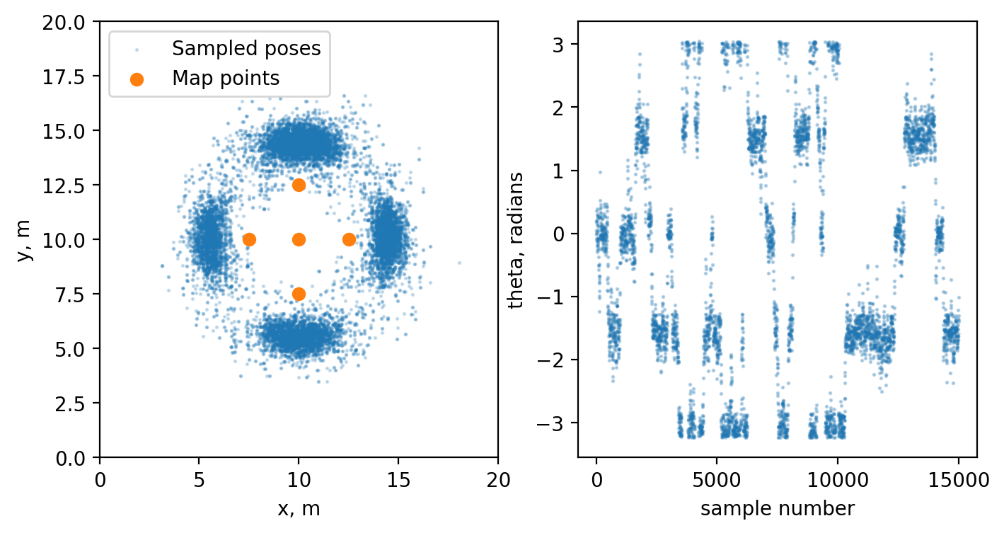
Option 2 Link to heading
Now let’s assume that we want to draw a lot of samples. What we can do is to precalculate the likelihood on a grid and directly sample from our conditional distribution.
import numpy as np
from scipy.spatial import KDTree
from scipy.stats import norm
import matplotlib.pyplot as plt

def norm_pdf(x, mu, sigma):
    """Calculates normal pdf for sample x given parameters mu and sigma."""
    variance = sigma**2
    numerator = x - mu
    denomenator = 2*variance
    pdf = ((1/(np.sqrt(2*np.pi)*sigma))*np.exp(-(numerator**2)/denomenator))
    return pdf

def transform_to_world(perception, pose):
    """Resolves perception in world coordinate frame based on current pose."""
    x, y, theta = pose
    c, s = np.cos(theta), np.sin(theta)

    perception_world = np.zeros_like(perception)
    for i, p in enumerate(perception):
        perception_world[i, :] = (p[0] * c - p[1] * s + x, p[0] * s + p[1] * c + y)

    return perception_world

def estimate_perception_logpdf(perception, x, y, theta, sigma=1.):
    """Calculates pdf of perception given the pose."""
    perception_world = transform_to_world(perception, (x, y, theta))
    distances, _ = tree.query(perception_world, k=1)
    w = np.sum(np.log(norm_pdf(distances, 0., sigma)))
    return w

def normalized_weights(taus):
    """Used to normalize and converts weights to normal scale"""
    max_tau = taus.max()
    return np.exp(taus - max_tau - np.log(np.sum(np.exp(taus - max_tau))))

def get_logpdf_on_a_grid(perception):
    """Get PDF on a grid"""
    # used to map x to idx on a grid
    x_to_idx = {x:i for i, x in enumerate(np.arange(0, 20., 0.25))}
    y_to_idx = {y:i for i, y in enumerate(np.arange(0, 20., 0.25))}
    theta_to_idx = {theta:i for i, theta in enumerate(np.deg2rad(np.linspace(-180, 180 - 180/16, 32)))}

    logpdf_xytheta = np.zeros((len(x_to_idx), len(y_to_idx), len(theta_to_idx)))
    for x in x_to_idx.keys():
        for y in y_to_idx.keys():
            for theta in theta_to_idx.keys():
                logpdf_xytheta[x_to_idx[x], y_to_idx[y], theta_to_idx[theta]] = estimate_perception_logpdf(perception, x, y, theta)

    return logpdf_xytheta, x_to_idx, y_to_idx, theta_to_idx

def sample_from_conditional_logpdf(conditional_logpdf, values_to_sample_from):
    # first sample the bin given bin weights
    bin_center = np.random.choice(values_to_sample_from, size=1, p=normalized_weights(conditional_logpdf))[0]
    # then sample actual value inside bin
    bin_width = values_to_sample_from[1] - values_to_sample_from[0]
    sample = np.random.uniform(bin_center - bin_width/2, bin_center + bin_width/2)
    return sample

# Define world points
map_points = np.array([[10., 7.5], [7.5, 10.], [10., 10.], [12.5, 10.], [10., 12.5]])
tree = KDTree(map_points)
# Define robot perception of the world
perception = [[2., 0], [4.5, -2.5], [4.5, 0.], [4.5, 2.5], [7., 0]]

logpdf_xytheta, x_to_idx, y_to_idx, theta_to_idx = get_logpdf_on_a_grid(perception)

current_pose = (np.random.uniform(0, 20), np.random.uniform(0, 20), np.random.uniform(-np.pi, np.pi))
samples = [current_pose]
xx, yy, tt = np.array(list(x_to_idx.keys())), np.array(list(y_to_idx.keys())), np.array(list(theta_to_idx.keys()))
for i in range(0, 5000):
    x, y, theta = samples[-1]
    # find the conditional pdf row, column given current y coordinate and theta angle
    y_idx, theta_idx = np.abs(yy - y).argmin(), np.abs(tt - theta).argmin()
    # sample from logpdf_x_given_ytheta
    sampled_x = sample_from_conditional_logpdf(logpdf_xytheta[:, y_idx, theta_idx], xx)
    samples.append((sampled_x, y, theta))

    x, y, theta = samples[-1]
    # find the conditional pdf row, column given current x coordinate and theta angle
    x_idx, theta_idx = np.abs(xx - x).argmin(), np.abs(tt - theta).argmin()
    # sample from logpdf_y_given_xtheta
    sampled_y = sample_from_conditional_logpdf(logpdf_xytheta[x_idx, :, theta_idx], yy)
    samples.append((x, sampled_y, theta))

    x, y, theta = samples[-1]
    # find the conditional pdf row, column given current x and y coordinates
    x_idx, y_idx = np.abs(xx - x).argmin(), np.abs(yy - y).argmin()
    # sample from logpdf_theta_given_xy
    sampled_theta = sample_from_conditional_logpdf(logpdf_xytheta[x_idx, y_idx, :], tt)
    samples.append((x, y, sampled_theta))


fig, ax = plt.subplots(1, 2, figsize = (8, 4))
samples = np.array(samples)
ax[0].scatter(samples[:, 0], samples[:, 1], s=1, alpha = 0.2, c="tab:blue", label="Sampled poses")
ax[0].scatter(map_points[:, 0], map_points[:, 1], c='tab:orange', label="Map points")
ax[0].set(xlim=(0, 20), ylim=(0, 20), xlabel="x, m", ylabel="y, m")
ax[0].legend()
ax[1].scatter(np.arange(0, len(samples)), samples[:, 2], s=1, alpha = 0.1, c="tab:blue", label="Sampled poses theta")
ax[1].set(xlabel="sample number", ylabel="theta, radians")
References Link to heading
[1]: https://www.bishopbook.com/, Ch. 14.