Notes on Computer vision
Notes on Computer vision Link to heading
I have made these notes while reading Computer vision: Models, Learning, and Inference book.
Coordinate systems notation Link to heading
$\mathbf{R}_{wc}$ is a rotation matrix such that, after its application to the camera axes, they become collinear with the world axes. Some describe it as a matrix that rotates a vector from the camera coordinate system to the world coordinate system. However, this description can be slightly misleading, as vectors exist in space and are not physically rotated. $\mathbf{t}_{wc}$ is a translation vector from the origin of the world axes to the origin of the camera axes; if we apply this translation to the point associated with the origin of the world coordinate system, it will coincide with the point associated with the origin of the camera coordinate system.
Now, if we want to determine the position of a point known in the camera coordinate system in terms of the world coordinate system, we can apply the following transformation: $\mathbf{p}_w = \mathbf{R}_{wc} \mathbf{p}_c + \mathbf{t}_{wc}$.
Also, note that $\mathbf{t}_{wc} = -\mathbf{R}_{wc}\mathbf{t}_{cw}$ (can be easily derived from the equations describing the $(\mathbf{R}_{cw}, \mathbf{t}_{cw})$ and $(\mathbf{R}_{wc}, \mathbf{t}_{wc})$ transformations applied to two points).
Because of the vector addition the aforementioned transformation expression is not linear, also stacking these transformation becomes a tedious task. So it is more useful to combine both Rotational and translation parts into one matrix, this matrix allows to work on homogeneous coordinates (we transform 3D vector to homogeneous one by adding one element at the end). Then such a vector could be transformed using transformation matrix $\mathbf{T}_{wc}$. This matrix has a special form and set of all these matrices is known as $SE(3)$ group.
Transformation types Link to heading
Most common transformations types
| Transform | Matrix | DoF | Invariance | Eigen:: class |
|---|---|---|---|---|
| Euclidian | $$\begin{bmatrix}\mathbf{R} & \mathbf{t} \\ \mathbf{0}^T & 1\end{bmatrix}$$ | 6 | Length, angle, volume | Matrix3d, AngleAxisd |
| Similarity | $$\begin{bmatrix}s\mathbf{R} & \mathbf{t} \\ \mathbf{0}^T & 1\end{bmatrix}$$ | 7 | angle, volume ratio | Isometry3d |
| Affine | $$\begin{bmatrix}\mathbf{A} & \mathbf{t} \\ \mathbf{0}^T & 1\end{bmatrix}$$ | 12 | parallelism, volume ratio | Affine3d |
| Perspective | $$\begin{bmatrix}\mathbf{A} & \mathbf{t} \\ \mathbf{a}^T & v\end{bmatrix}$$ | 15 | intersections, tangency | Projective3d |
Camera model Link to heading
Key terms Link to heading
Pinhole camera model - closed chamber with a small hole, rays from an object pass through the hole and form an inverted image. To avoid inversion the virtual image is usually used, that would result from placing an image between the pinhole and the object.
Pinhole model - generative model that describes the likelihood $Pr(\mathbf{x}|\mathbf{w})$ of observing a feature at position $\mathbf{x} = [x, y]^T$ in the image given that it is the projection of a 3D point
$$\mathbf{w} = [u, v, w]^T$$in the the world.
Principal point - point where optical axis of the camera strikes the image plane.
Focal length - distance between optical center of the camera and principal point.
Perspective projection - the process of finding the position of the point, expressed in world coordinate frame, on the image plane. The usual way to do so is to connect a ray between $\mathbf{w}$ and the optical center, the image position $\mathbf{x}$ can be found by observing where this ray strikes the image plane.
Normalized camera - the camera, which focal length is one, and the origin of the 2D image coordinate system is at the principal point. In the normalized camera, $\mathbf{w}$ is projected into the image at $\mathbf{x}$ using the following relations:
$$ \begin{equation} \begin{split} x &= \frac{u}{w}\\ y &= \frac{v}{w}, \end{split} \end{equation} $$and all values are measured in the same real-world units. If the camera coordinates are multiplied by any non-zero number, the normalized coordinates are the same. This means that the depth information is lost during the projection process.
The defined model assumes that the image coordinate center is located at the principal point. Quite often, however, the origin should be at the top-left of the image. To account for this, the model enriches with the parameters $\delta_x$ and $\delta_y$. They are the offsets, or positions of the principal point in pixels, measured from top-left corner of the image. Another parameter is skew, $\gamma$, it has no clear physical interpretation, but can help to explain the projection of points. The resulting camera model is
$$ \begin{equation} \begin{split} x &= \frac{\phi_x u + \gamma v}{w} + \delta_x\\ y &= \frac{\phi_y v}{w} + \delta_y. \end{split} \end{equation} $$Full pinhole camera model Link to heading
The standard way is to separate the model parameters into two sets:
- intrinsic, or camera parameters: $\{\phi_x, \phi_y, \gamma, \delta_x, \delta_y\}$, that describe camera itself.
- extrinsic parameters: $\{ \boldsymbol{\Omega}, \boldsymbol{\tau} \}$, or $\{ \mathbf{R}_{cw}, \mathbf{t}_{cw} \}$ to express the world points in the coordinate system of the camera before they are passed through the projection model.
Usually the intrinsic parameters are gathered in intrinsic matrix $\boldsymbol{\Lambda}$:
$$ \boldsymbol{\Lambda} = \begin{bmatrix} \phi_x & \gamma & \delta_x \\ 0 & \phi_y & \delta_y\\ 0 & 0 & 1 \end{bmatrix}, $$then the full pinhole camera model can be abbreviated as:
$$ \mathbf{x} = \text{pinhole}[\mathbf{w}, \boldsymbol{\Lambda}, \boldsymbol{\Omega}, \boldsymbol{\tau}]. $$To account for uncertainty when the estimated position of the feature differs from our predictions, we can use spherically isotropic noise:
$$ Pr(\mathbf{x}|\mathbf{w}, \boldsymbol{\Lambda}, \boldsymbol{\Omega}, \boldsymbol{\tau}) = \text{Norm}_{\mathbf{x}}[\text{pinhole}[\mathbf{w}, \boldsymbol{\Lambda}, \boldsymbol{\Omega}, \boldsymbol{\tau}], \sigma^2\mathbf{I}]. $$It is generative model, that describes the likelihood of observing a 2D image point $\mathbf{x}$ given the 3D world point $\mathbf{w}$ and the parameters $\{\boldsymbol{\Lambda}, \boldsymbol{\Omega}, \boldsymbol{\tau}\}$.
Distortion Link to heading
To get a larger FoV one usually adds a lens in front of the camera. Usually there are two types of distortions: first comes because of the lens shape and is called radial distortion, second one is the result of misalignment between the lens plane and image surface.
Radial Link to heading
It is the nonlinear warping of the image that depends on the distance from the center of the image. U Radial distortion is modeled as a polynomial function of the distance from the center of the image. The final positions are expressed as functions of the original ones:
$$ \begin{split} x' = x(1 + \beta_1 r^2 + \beta_2 r^4) \\ y' = y(1 + \beta_1 r^2 + \beta_2 r^4). \end{split} $$This distortion is implemented after perspective projection (division by $w$) but before the effect of the intrinsic parameters (focal length, offset, etc.).
Undistortion Link to heading
To make undistortion two approaches could be used:
- We go through the undistorted image pixels and calculate its distorted position, copying the pixel from distorted image to an undistorted one. We can directly use the aforementioned equation.
- We know the positions of distorted pixels and want to find their positions on an undistorted image. To do so we need numerically find the solution of the aforementioned equations.
Three geometric problems Link to heading
These three problems is the an extraction from [2, pp. 304-306].
Problem 1: Learning extrinsic parameters Link to heading
Problem: recover the position and orientation of the camera relative to a known scene. This is known as the perspective-n-point (PnP) problem or the exterior orientation problem.
We are given a set of $I$ distinct 3D points $\{ \mathbf{w}_i \}_{i=1}^{I}$, their corresponding projections in the image $\{ \mathbf{x}_i \}_{i=1}^{I}$ and known intrinsic parameters $\boldsymbol{\Lambda}$. Goal - estimate the rotation and translation that map points in the coordinate system of the object to points in the coordinate system of the camera so that:
$$ \hat{\boldsymbol{\Omega}}, \hat{\boldsymbol{\tau}} = \argmax_{\boldsymbol{\Omega}, \boldsymbol{\tau}} \left[ \sum_{i=1}^{I}\log \left[ Pr(\mathbf{x}_i | \mathbf{w}_i, \boldsymbol{\Lambda}, \boldsymbol{\Omega}, \boldsymbol{\tau}) \right]\right] \\ = \argmax_{\boldsymbol{\Omega}, \boldsymbol{\tau}} \left[ \sum_{i=1}^{I}\log \left[ \text{Norm}_{\mathbf{x}_i}\left[\text{pinhole}[\mathbf{w}_i, \boldsymbol{\Lambda}, \boldsymbol{\Omega}, \boldsymbol{\tau}], \sigma^2\mathbf{I} \right] \right]\right] $$This is a maximum likelihood learning problem, where we aim to find parameters $\boldsymbol{\Omega}, \boldsymbol{\tau}$ that make the predictions $\text{pinhole}[\mathbf{w}, \boldsymbol{\Lambda}, \boldsymbol{\Omega}, \boldsymbol{\tau}]$ of the model agree with the observed 2D points.
Problem 2: Learning intrinsic parameters, calibration Link to heading
This problem is known as calibration. The inputs are the same. Usually the calibration target is used to construct the points.
$$ \hat{\boldsymbol{\Lambda}} = \argmax_{\boldsymbol{\Lambda}}\left[ \max_{\boldsymbol{\Omega}, \boldsymbol{\tau}} \left[ \sum_{i=1}^{I}\log \left[ Pr(\mathbf{x}_i | \mathbf{w}_i, \boldsymbol{\Lambda}, \boldsymbol{\Omega}, \boldsymbol{\tau}) \right]\right] \right ]. $$Problem 3: Inferring 3D world points, triangulation Link to heading
Problem: estimate the 3D position of a point $\mathbf{w}$ in the scene, given its projections $\{ \mathbf{x}_j\}_{j=1}^{J}$ in $J\geq 2$ calibrated cameras. When $J=2$, this is known as a calibrated stereo reconstruction. With $J>2$ calibrated cameras, it is known to as multiview reconstruction. If the process is repeated for many points, the result is a sparse 3D point cloud.
Formal description: given $J$ calibrated cameras in known positions, viewing the same 3D point $\mathbf{w}$ and knowing the corresponding 2D projections $\{ \mathbf{x}_j\}_{j=1}^{J}$ in the $J$ images establish the 3D position $\mathbf{w}$ in the world:
$$ \hat{\mathbf{w}} = \argmax_{\mathbf{w}} \left[ \sum_{j=1}^{J}\log \left[ Pr(\mathbf{x}_j | \mathbf{w}, \boldsymbol{\Lambda}_j, \boldsymbol{\Omega}_j, \boldsymbol{\tau}_j) \right]\right]. $$The principle behind reconstruction is known as triangulation.
Two-view camera geometry Link to heading
Key terms Link to heading
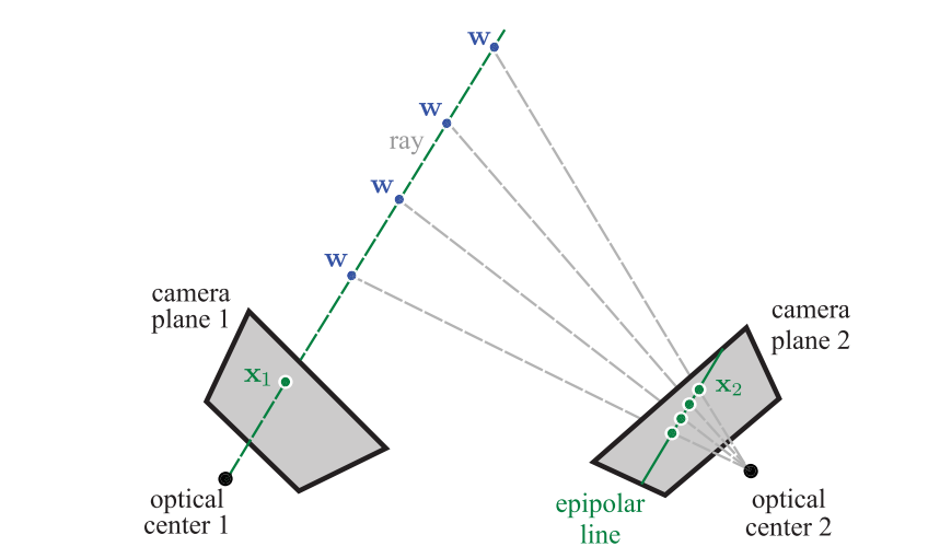 Epipolar line - the line in the image plane of one camera that corresponds to the projection of a 3D ray coming out of the optical center of another camera.
Epipolar constraint - for any point in the first image, the corresponding point in the second image is constrained to lie on a line.
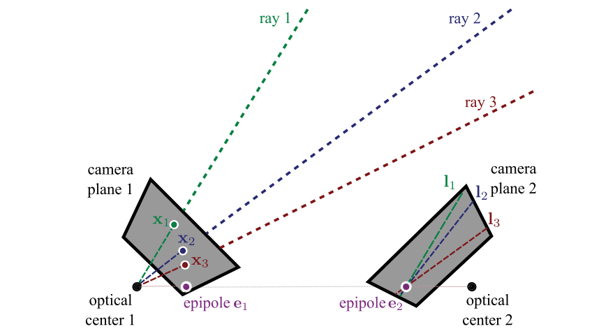 Epipole - a single point where all epipolar lines converge. It is the image in the second camera of the optical center of the first camera.
The essential matrix Link to heading
An arbitrary 3D point $\mathbf{w}$ is projected into the cameras as:
$$ \begin{split} \lambda_1 \tilde{\mathbf{x}}_1 &= [\mathbf{I}, \mathbf{0}]\tilde{\mathbf{w}} \\ \lambda_2 \tilde{\mathbf{x}}_2 &= [\mathbf{\Omega}, \boldsymbol{\tau}]\tilde{\mathbf{w}}. \end{split} $$Here it is assumed that the cameras are normalized ($\mathbf{\Lambda}_1 = \mathbf{\Lambda}_2 = \mathbf{I}$), $\lambda$ - arbitrary scale factors (any scalar multiple $\lambda$ represents the same 2D point). Now, having the same point observed in the first and second camera, and both are expressed in homogeneous coordinate, we have:
$$ \begin{split} \lambda_1 \tilde{\mathbf{x}}_1 &= \mathbf{w} \\ \lambda_2 \tilde{\mathbf{x}}_2 &= \mathbf{\Omega} \mathbf{w} + \boldsymbol{\tau}. \end{split} $$Substituting first into second:
$$ \lambda_2 \tilde{\mathbf{x}}_2 = \mathbf{\Omega} \lambda_1 \tilde{\mathbf{x}}_1 + \boldsymbol{\tau}. $$This is the expression that represents a constraint between the possible positions of the corresponding points in two images. It is only parametrized by the transform of the second camera relative to the first. After some manipulations ([2], p. 360) we can get that:
$$ \tilde{\mathbf{x}}_2^T \mathbf{E} \tilde{\mathbf{x}}_1 = 0, $$where $\mathbf{E} = \boldsymbol{\tau}{\times}\mathbf{\Omega}$ is known as the essential matrix. This relation is the math constraint between the positions of corresponding points in two normalized cameras.
The fundamental matrix Link to heading
In the essential matrix it is assumed that the normalized camera models are used ($\boldsymbol{\Lambda}_1 = \boldsymbol{\Lambda}_2 = \mathbf{I}$). The fundamental matrix is the same as the essential matrix for cameras with arbitrary intrinsics matrices $\boldsymbol{\Lambda}_1$ and $\boldsymbol{\Lambda}_2$.
The contraint imposed by the fundamental matrix has the following form:
$$ \tilde{\mathbf{x}}_2^T \mathbf{F} \tilde{\mathbf{x}}_1 = 0, $$where $\mathbf{F} = \boldsymbol{\Lambda}_2^{-T} \mathbf{E} \boldsymbol{\Lambda}_1^{-1}$ is the fundamental matrix, and $\tilde{\mathbf{x}}_1$ and $\tilde{\mathbf{x}}_2$ are the normalized image coordinates of the corresponding points in the two images.
As a result, the essential matrix can be recovered from the fundamental matrix by the following equation:
$$ \mathbf{E} = \boldsymbol{\Lambda}_2^T \mathbf{F} \boldsymbol{\Lambda}_1. $$Two-view reconstruction pipeline Link to heading
The rudimentary pipeline for 3D scene reconstruction consists of the following steps:
- Compute image features.
- Compute feature descriptors.
- Find initial matches:
- by computing the squared distance between the descriptors and checking that it exceeds a predefined threshold to filter out false matches;
- by rejecting matches where the ratio between the quality of the best and second best match is close (identifying that alternative matches are plausible).
- Compute fundamental matrix.
- Refine matches using the fundamental matrix and epipolar geometry.
- Estimate essential matrix
- Decompose essential matrix to obtain the relative camera pose.
- Estimate 3D points.
Rectification Link to heading
Process of aligning two images so that corresponding points lie on the same horizontal line in both images.